Day 42: the benchmark, and the queue a closed loop cannot see

Date: 2026-08-23 · Week 12 · Phase 5 Benchmark and optimize

What I added today

servebench.py, twice: nanoserve.servebench is the measurement, and the root script is the flags. The module has RequestRecord (one request’s whole timeline as timestamps, with TTFT, the frame gaps and the two end-to-end numbers derived off it), LoadReport (the run’s window, its rates, its percentiles and mean_in_flight), percentile (nearest rank), the three arrival schedules burst_arrivals / fixed_arrivals / poisson_arrivals, the two drivers run_open_loop and run_closed_loop, and the two checks a benchmark owes itself, check_offered_load and check_schedule_kept, which raise MeasurementUnsound. tests/test_servebench.py is 28 tests: the arithmetic against a scripted timeline, then the drivers against a real uvicorn on a real port, reusing Day 41’s live_server and ClientPlan. Suite 759 green (5 GPU-gated skips), ruff clean.

The real Llama-3.2-1B, cpu fp32, 2 slots, 16-token answers, Poisson arrivals, ten requests per rate:

offered   achieved   in flight   tok/s   TTFT p50   TTFT p99   ITL p50
0.1 rps      0.11       1.28      1.8       2.42s      4.96s     610ms
0.2 rps      0.16       2.83      2.5       5.23s     18.72s     610ms
0.4 rps      0.16       4.48      2.5      17.49s     34.54s     611ms
0.8 rps      0.16       5.28      2.5      22.26s     44.47s     609ms

and the same server, driven the two different ways, on the same eight requests:

closed loop, 2 clients   2.6 tok/s   TTFT p50  2.34s   p99  3.79s
open loop, all at once   2.8 tok/s   TTFT p50 14.20s   p99 37.02s

Why it matters

The load generator decides what you are allowed to find out. A closed loop keeps N clients busy: each sends its next request when its last one comes back. It is the natural thing to write and it has one property that disqualifies it from measuring latency, which is that the load it offers falls when the server slows down. Double the service time and the same clients send half as many requests per second, so the server is never asked to hold a queue, so the TTFT it reports is its service time with the queueing removed. That is Gil Tene’s coordinated omission, and in a serving system it removes almost all of the answer, because almost all of the wait is the wait for a slot.

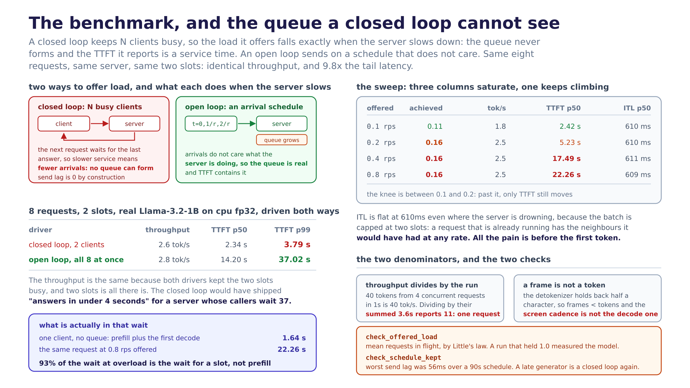
The two rows above are the same eight requests against the same server. Throughput is the same to within noise, 2.6 against 2.8 tokens per second, because both drivers kept the two slots busy and two slots is all there is. The p99 time to first token differs by 9.8x. A closed-loop benchmark would have reported this server as answering in under four seconds while its actual callers, arriving when they felt like it rather than when it was ready, waited thirty-seven.

The knee is a rate, and only an open loop has one. The sweep is the shape worth knowing: achieved rate rises to 0.16 requests per second and then stops, because that is what the box can do, and every rate offered above it produces the same 0.16. Throughput stops at 2.5 tokens per second at the same moment. Neither of those two numbers can tell 0.2 rps from 0.8 rps. TTFT can: 5.2 seconds against 22.3. Past saturation the only variable left is how long the queue is, so a benchmark that reports throughput alone reports a server that is behaving identically at four times the load, while its users are waiting four times longer.

The ITL column is flat, and that is the finding, not the control. 610ms at every rate including the ones where the server is drowning. The batch is capped at two slots, so a request that is running has exactly the neighbours it would have had at any other rate: the overload cannot reach it. All of the cost lands before the first token and none of it lands between tokens. That is a property of an admission-limited engine and it is worth knowing, because the intuition “the server is overloaded so everything gets slower” predicts the opposite, and would have sent me looking for a decode regression that does not exist.

Two denominators that quietly ruin a report. The first is throughput: forty tokens delivered by four concurrent requests inside one second is forty tokens per second, and dividing by the 3.6 seconds those four requests collectively spent in flight gives 11, which is one request’s rate wearing the run’s name. output_tps divides by the run window. The summed residency is kept anyway, as mean_in_flight, because by Little’s law it is the average number of requests in the system, and it is this module’s admissibility instrument: check_offered_load refuses a report below a floor, since a run that held 1.0 requests measured the model and called it the server. It is Day 41’s peak_running on the client’s side of the socket.

The second is the token count. The stream is the only endpoint that can be timed per token, because a unary response arrives in one piece, so a “latency” measured there has no TTFT and no cadence in it at all and looks excellent. But the frames a client counts are not the tokens the engine produced: Day 39’s incremental detokenizer holds a token back when it is half a UTF-8 character, and the server does not emit an empty frame. So median_itl_s is the frame cadence, which is what the reader’s screen did, mean_token_itl_s is the decode span over the real token count from the usage bill, which is what the engine did, and the two differ by exactly tokens_per_frame. The terminal frame is excluded from both: it carries finish_reason and the bill, and counting it as a token adds a gap that no token caused.

And the harness can be the bottleneck, so it reports on itself. An open loop is only open while it keeps its schedule. A generator that sends late stopped offering load exactly when the server got slow, which is coordinated omission arriving through the back door, and the symptom is a latency graph that improves as the server degrades. So every record carries send_lag_s, the gap between when a request was due and when it actually left, and check_schedule_kept refuses a report that fell behind. The worst lag in the sweep above was 56ms against a 90 second schedule. On a closed-loop report that lag is exactly zero, by construction, because there is no schedule to fall behind, and printing that zero next to the open loop’s is the clearest way I have found to say what the closed loop is not measuring.

What I learned

1. The unloaded number is the one to subtract. One client on this box gets a TTFT of 1.64s, which is the prompt’s prefill plus the first decode and nothing else. At 0.8 rps offered the same request waits 22.26s. The difference, 20.6 seconds, is queueing: 93% of the wait at overload is the wait for a slot, and no amount of prefill optimization touches it. That subtraction is the cheapest version of “separate queueing from prefill” available from outside the process, and it is why the split is worth doing properly server-side tomorrow rather than guessing which half to optimize.
2. Batching costs cadence, and on this box it buys nothing back. ITL goes 341ms at one row to 610ms at two, a 1.79x tax, while throughput goes 2.4 to 2.5 tokens per second, a 4% gain. That is Day 29’s measurement arriving over HTTP: decode is memory-bound on a card, where a second row rides along in arithmetic that was idle anyway, and CPU fp32 is arithmetic-bound, where it does not. The tradeoff that makes continuous batching correct is a hardware ratio, and this box has the wrong one. Worth stating plainly every time a number from it is quoted.
3. Poisson arrivals, not evenly paced ones. A fixed interval is the gentlest possible load at a given rate: a server whose service time fits inside the interval never sees two requests at once, so it reports a queue-free latency right up until it saturates and then falls off a cliff. Exponential gaps are memoryless, so short gaps are common, and requests land on top of each other even at rates well under capacity. That is the tail production has. Seeded, because a benchmark that fails at a rate and passes at the same rate ten minutes later has told me nothing.
4. Nearest-rank percentiles, and n printed next to every one. An interpolated p99 can be a latency no caller experienced, which is fine for a distribution and wrong for a report about what happened to people. And with ten samples, ceil(0.99 * 10) is 10: the p99 is the maximum, wearing a name it has not earned. Every percentile in summary() prints its sample count for that reason. The 44.47s p99 above is the worst of ten, and honest only as that.
5. A p99 past the knee is a fact about the run’s length, not about the server. Once arrivals outrun service the queue never drains, so latency grows for as long as the run continues: those ten requests at 0.8 rps would have reported a worse tail at twenty and worse again at fifty. The rates below the knee are the ones that can be quoted as capacity. The ones above it are the shape of the wall, and the number to take from them is where the wall is.
6. A 200 that delivered nothing is not a success. RequestRecord.ok requires a frame, not just a status, because a request with no first token has no TTFT, and letting it into the percentiles as a zero drags every one of them down towards a latency nobody had. It belongs in n_failed, where somebody will ask about it. The same reasoning put the pooled ITL count in the report: 150 frame gaps from 10 requests, weighted towards whoever generated the most tokens, which is the right weighting for a question about tokens and the wrong one for a question about requests.

Diagram

open-loop-latency.png. Left top is the two generators, with what each one does when the server slows down. Left bottom is the same eight requests driven both ways: identical throughput, 9.8x the p99. Right top is the rate sweep as the knee, with the three columns that saturate and the one that does not. Right bottom is the vocabulary, the two denominators, and the two checks.

Tomorrow

Day 43 puts the split that today had to estimate inside the server: an arrival, an admission and a first-token timestamp on the Request itself, so TTFT comes apart into queue wait, prefill and first decode as a measurement rather than as the 1.64-second subtraction above. Then the baseline the week is really for, which is the same prompts and the same box through HuggingFace generate, one request at a time because that is all it can do, against this engine’s numbers. That comparison is the only one that says whether the paged cache and the scheduler bought anything real, and it needs today’s harness on both sides so the two are measured with the same definitions.

Post angle

Day 42 of building an LLM inference engine from scratch. Benchmarked the server for the first time, and the first thing I measured was my benchmark. There are two ways to drive load. A closed loop keeps N clients busy, each sending the next request when the last one returns. It is what most homegrown benchmarks are, and it cannot measure latency, because the load it offers falls when the server slows down: twice the service time means half the requests per second from the same clients, so the queue never forms and the TTFT you report is the service time with the queueing removed. Gil Tene calls it coordinated omission. In a serving system it removes almost the whole answer, because almost the whole wait is the wait for a slot. Same eight requests, same server, two slots, real Llama-3.2-1B on CPU: closed loop reports 2.6 tok/s and a p99 TTFT of 3.79s. Open loop, requests arriving on a schedule that does not care what the server is doing, reports 2.8 tok/s and a p99 TTFT of 37.0s. Same throughput, 9.8x the tail. Then the sweep, which is the shape worth having: offered 0.1, 0.2, 0.4, 0.8 requests per second, and achieved stops at 0.16 and stays there. Throughput stops at 2.5 tok/s and stays there. Neither can tell 0.2 from 0.8. TTFT p50 can: 5.2s against 22.3s. And the inter-token latency is 610ms at every single rate, because the batch is capped at two, so an overloaded server cannot reach a request that is already running. All the pain is before the first token, none of it is between tokens. 759 green.