Day 29: static batching, measured

Date: 2026-07-23 · Week 7 · Phase 3 Batching and scheduler

What I added today

src/nanoserve/batchbench.py, the instrument that says what Week 7 actually bought. BatchTiming holds one static-batch run (the prefill, one duration per decode step, and per row the number of steps that row’s own generation needed) and derives the two costs a fixed batch pays. issued_tokens is what the forward computed, useful_tokens is what a row collected, and waste_fraction is the gap: throughput spent on rows that had already finished. hol_delay_s, hol_inflation and max_hol_inflation are the other cost, latency: a static batch hands every row back when its slowest row is done, so a row that finished early holds an answer nobody is allowed to have yet. BatchScaling and fit_batch_scaling take the other measurement, goodput against batch size, with speedup, efficiency (the share of ideal linear scaling that survived) and knee (the largest size still paying its way).

The timing core is stdlib-only with the clock injected, the split Day 13 drew and Day 20 repeated. The runner below it is the Day-26 treatment: build_batched_decode stands up a real BatchedPagedKVCache, runs the Day-27 padded prefill and the Day-28 batched decode step, and hands the core two closures, so the sweep times the loop greedy_generate_batch runs rather than a function called in isolation. A test pins that the tokens it collects are exactly that method’s output. Rows stop on a step budget rather than on EOS, because raggedness is the variable being swept and output length is a property of the prompt; every forward is real and a finished row keeps its query, its slot and its block.

batchbench.py at the repo root runs both measurements and writes docs/daily/data/day-29-batchbench.csv. Forty new tests across tests/test_batchbench.py (pure, fake clock) and tests/test_batchbench_model.py (real model, real pool). Suite 279 green (5 GPU-gated skips), ruff clean.

Why it matters

Week 7’s code is done and its claim was untested. “Batching is the difference between using the card and paying for it” has been in batch.py’s docstring since Day 27 as an argument, and Week 8 is justified entirely by where that argument stops holding, so it had to become numbers.

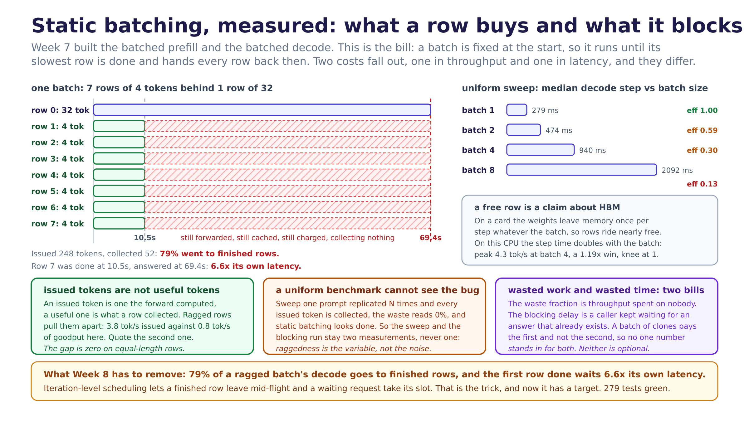
The blocking run is the number Week 8 exists to remove. Seven rows of 4 tokens batched behind one row of 32: the decode issues 248 tokens and collects 52, so 79% of the forward was computed for rows that were already done, and goodput is 0.8 tok/s against an issued 3.8 tok/s. The latency half is worse than the throughput half. A short row’s own work ended at 10.5s and its answer was returned at 69.4s: 6.6x its own latency, 58.9s of which was dead time holding a finished result. Those are two separate bills and this module refuses to average them, because a fix that recovers the wasted compute without releasing the finished row still leaves a user waiting 6.6x too long.

The sweep is the part that did not go the way the docstring promised, and that is the more useful result. On this CPU the median decode step goes 279ms, 474ms, 940ms, 2092ms for batches of 1, 2, 4 and 8: efficiency 1.00, 0.59, 0.30, 0.13. Peak goodput is 4.3 tok/s at batch 4, a 1.19x win over one sequence, and the knee is already at batch 1. The whole “another row is nearly free” argument is a claim about HBM bandwidth (the weights are read out of memory once per step whatever the batch, so the extra rows ride along in arithmetic that was idle anyway), and it is only true on hardware where that read is the bottleneck. This box has no HBM and its fp32 matmuls are compute-bound, so a second row costs most of a second step. Same numbers on the real Llama-3.2-1B as on the random weights, which is the expected result: the shapes are identical and only the shapes matter. The instrument is right and the hardware is what it is, and I would rather ship a benchmark that reports 1.19x on the box it ran on than one tuned until it agrees with the marketing.

What I learned

1. A uniform benchmark cannot see the thing static batching is bad at. The first version of the sweep was the only measurement I planned: replicate one prompt N times, time the decode, plot tokens per second. Every row in that batch is the same length, so every issued token is collected, waste_fraction reads exactly 0.0, and static batching looks finished. The failure mode only exists when output lengths differ, so raggedness has to be a swept variable rather than something the prompt set happens to have. That is why the module ended up with two entry points that are never averaged: sweep_batch_sizes for what a row buys, time_model_batch with a stop_steps for what it blocks. A benchmark that reports one number for both is not being conservative, it is hiding the half it cannot see.
2. “Issued” and “useful” needed to be two words before I could measure anything. I started with a single tokens_per_s and could not make it mean anything: the batch computes batch_size tokens every step, and on a ragged batch that is not what anyone received. Both counts are real, they describe different things (what the hardware moved versus what the service delivered), and the ratio between them is exactly the quantity in question. Once they had separate names the head-of-line arithmetic wrote itself, and the same distinction is what production stacks mean by goodput. Naming the two halves was most of the design.
3. The memory-bound argument for batching is hardware-conditional, and I had been repeating it as if it were arithmetic. I expected efficiency near 1.0 up to batch 8 and got 0.13, and my first instinct was that the benchmark was wrong. It was not: a decode step is only memory-bound when reading the weights dominates computing with them, which is a statement about a specific ratio on specific hardware, not a property of transformers. On a CPU with fp32 GEMMs the arithmetic dominates and batch size buys only the per-step Python and allocation overhead, which is the 1.19x that showed up. The useful part is that head-of-line blocking is not hardware-conditional in the same way: the 79% waste and the 6.6x inflation are counts of steps and rows, so they hold on any box. Week 8’s case does not depend on having a card, which is worth knowing before building a scheduler on a machine without one.

Diagram

static-batching-measured.png. Left is the blocking run as a timeline: one long row spanning the batch, seven short rows finishing at 10.5s and then hatched red to 69.4s, still forwarded and still cached and collecting nothing, with the dashed line where every row is finally returned. Right is the uniform sweep, median decode step per batch size with its efficiency, and the note that a free row is a claim about HBM. The three boxes are the day’s lessons: issued against useful, why a uniform benchmark is blind here, and the two bills. The banner is the target Week 8 now has.

Tomorrow

Week 8 opens: the waiting and running queues, the first half of an iteration-level scheduler. The state a request is in (waiting, running, finished) becomes an object rather than an index into a fixed batch, which is the structural change that lets a finished row leave and a waiting one take its slot. Today’s numbers are the acceptance test for the week: rerun the blocking measurement against a scheduled loop and the waste fraction and the inflation both have to fall, on the same box, from the same harness. One debt carried forward from Day 28 and still unpaid: the batched paged read is a reference that gathers a [batch, max_ctx] rectangle, so a short row still pays for the longest row’s history. That is the Week 6 kernel treatment applied to the batch axis, and it is a speed change rather than a structural one, so it waits behind the scheduler.

Post angle

Day 29 of building an LLM inference engine from scratch. Week 7 gave me batched prefill and batched decode, so today I measured what that actually bought, and the interesting half is what it did not. Two numbers, and the mistake I nearly made was reporting one. Sweep a batch of identical prompts and static batching looks finished: every row is the same length, every token the forward computes is a token someone collected, the waste fraction reads 0.0. So I ran the case that a server actually sees, seven rows of 4 tokens batched behind one row of 32. The batch is fixed at the start, so it runs until its slowest row is done. The decode issued 248 tokens and collected 52, which means 79% of the forward was computed for rows that had already finished. Worse is the latency: a short row’s own work ended at 10.5s and its answer was handed back at 69.4s, 6.6x its own latency, with 58.9 of those seconds spent holding a result that already existed. Those are two different bills, wasted work and wasted time, and a batch of clones pays the first and not the second, which is exactly why one number cannot stand in for both. The other surprise was the throughput sweep. I had been repeating the standard line, another row in the batch is nearly free because decode is memory-bound, as if it were arithmetic. It is a claim about HBM bandwidth: the weights leave memory once per step whatever the batch, so extra rows ride along in arithmetic that was otherwise idle. This box has no HBM. On CPU fp32 the step time went 279ms, 474ms, 940ms, 2092ms for batches of 1, 2, 4 and 8, so efficiency fell to 0.13 and peak goodput was 1.19x at batch 4. The instrument is right and the hardware is what it is. The part that transfers anyway: head-of-line blocking is counted in steps and rows, not bandwidth, so the 79% and the 6.6x hold on any machine. That is the target continuous batching has to remove, and it is what vLLM and SGLang mean by scheduling at the iteration level instead of the batch. 279 green.